Analysis Independent Samples t-test

By means of an independent samples t-test for samples from two populations you test whether the population means of a certain variable for the two populations are equal or different. 
On this page we show you how to perform this t-test and also how to visualize the result.

The presentation takes the following steps:

• Hypotheses
• An interesting observation
• Asking for the test using SPSS
• The SPSS output for age by gender
• Checking for the equality of variances conditions
• Interpreting the rest of the output for age by gender
• The SPSS output for age by born where
• Interpreting the output for age by born where
• Graphical display of the results
• Download the sample data file

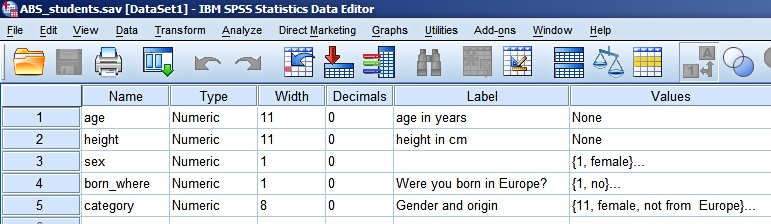
Note: In the section on testing you find some explananation of the method and way of thinking for testing of hypotheses.

Hypotheses:

For a number of years we have asked foundation year students to fill in a simple questionnaire with some questions about who they are. We use this data in class in our introductory statistics course. For this example we use the following data:

The original data have been slightly edited. Some people are outliers when age is concerned. They have been filtered out.
We are in this example interested in the differences in average age between groups. The first test investigates gender differences.

H₀: There are no differences between the average ages of female and male students from the foundation year of Arnhem Business School.
H_A: There are differences between the average ages of female and male students from the foundation year of Arnhem Business School.

Note: Since we have no indication about a direction for any difference in age, when comparing females and males, we perform a two-tailed test here.

The second difference to investigate is between people who were born in Europe and people not born in Europe.
In this case we suspect that students who were not born in Europe will be on average a little older when they come and study at Arnhem Business School (ABS) than the Europeans. So now we formulate the alternative hypothesis as one-tailed.

H₀: There are no differences between the average ages of students from the foundation year of ABS who are born in Europe versus those who aren't born in Europe .
H_A: On average students from the foundation year of ABS who are not born in Europe will be older than the students who are born in Europe.

An interesting observation

One of the questions of our little survey is: Were you born in Europe?  Yes / No.

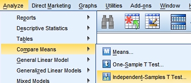
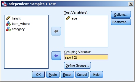
This sounds simple enough. What could possibly go wrong with it? Do you see any flaws in this question?
Now follow the link for a little surprise.

Asking for the test using SPSS

You specify the test variable, i.e. the variable for which the means will be calculated. In our example that is "age". You also have to specify which two groups are to be compared. You first choose the Grouping Variable and next you specify the two values that go with these groups. You see the groups definition for gender on the right. Note that you don't have to use two consecutive numbers. For the variable "born_where" we have "Group one = 1" and "Group two = 3".

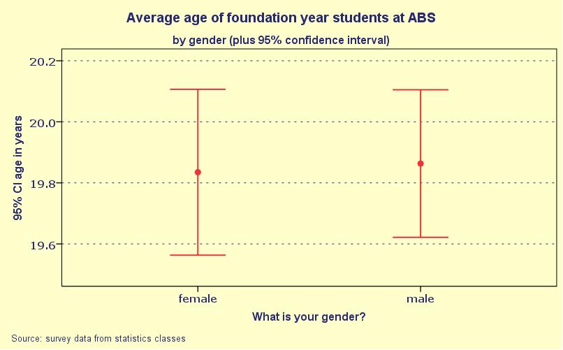
The SPSS output for age by gender

Checking the equality of variances condition

The original t-test assumed that the variable had equal variances for the two populations you wanted to compare. Later an extention has been deviced where this equality no longer was necessary. But to achieve this the formulas for the test statistic and the degrees of freedom of its t-distribution under H₀ has to be adjusted. Hence we now have two options to choose from. As you can see in the output above, SPSS has calculated both options and also provided us with the Levene test for equality of variances. The hypotheses for Levene are:

H₀:    The variances for age in the two populations (female and male foundation year students at ABS) are equal.
H_A:    The variances for age in the two populations are different

The Levene significance = 0.526 in our case, so we will stick with H₀for the Levene test. There are no indications that the variances are different.

Note: Looking at the Group Statistics in the output we see the standard deviations 2.063 (for females) and 1.965 (for males). There are almost equal, but we all know that small differences can nevertheless be statistically significant. So we need the test as well.

Interpreting the rest of the output for age by gender

We now know we can use the part labeled "Equal variances assumed". It gives us a two-tailed significance for the t-test of 0.877. Our conclusion is clear. There are no indications that the average ages for female and male foundation year students at ABS are different.

The 95% confidence interval for the difference tells us that it is between -0.39 and +0.33 years.

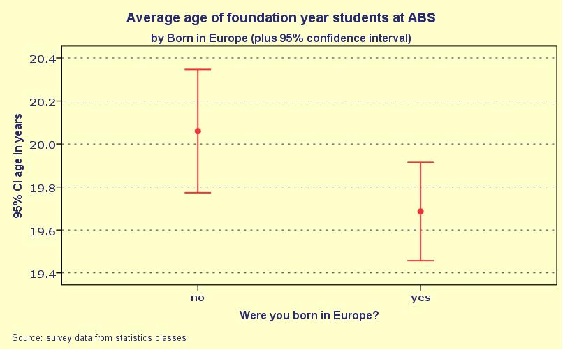
The SPSS output for age by "born where?"

We now come to the output for our second t-test. This one is formulated as one-tailed. We hypothesized that students coming from far away (from outside Europe) will be on average older than the students from Europe. Let's see what the data tells us.

Interpreting the output for age by "born where?"

Since we are dealing with a one-tailed test first of all we have to check whether or not the sample data is consistent with H_A. (If not, we can stop right away).
We see that the average age for students not born in Europe indeed is higher than for the Europeans (20.06 > 19.69).

Looking at the Levene test, we find a significance of 0.050. This is quite small; we play it save and reject the equality of variances. We will use the output from the line "Equal variances not assumed".

The two-tailed significance = 0.045. Hence the one-tailed significance = ½·0.045 = 0.0225. This is small enough to reject H₀.

Conclusion: There is considerable evidence that the average age for students not born in Europe is indeed higher than for the Europeans.

We can add to this the 95% confidence interval for the difference: On average the foundation year students from ABS not born in Europe are between 0.01 and 0.74 years older than the European born ones. The mean difference in age is 0.37 years.

Graphical display of the results

We are interested in differences in average age. And we have seen above that the variance of the dependent variable plays a role as well. To depict this situation an error bar chart is well suited. We choose it from the Legacy Dialogs:

We need a Simple Error Bar: Summaries for Groups of Cases. The dependent variable is "age". On the Category Axis we choose once "sex" and once "born_where". The bars represent Confidence interval for mean. The default confidence level of 95% is ok.

These pictures speak for themselves and nicely visualize our findings from the t-tests.